|
[Objectives | Exercises | Example
1 | Example 2 ]
OBJECTIVES
 | To become familiar with ode45, one of MATLAB's ODE
solvers. |
 |
Typing help ode45 gives the following information:
ODE45 Solve non-stiff differential equations, medium order method.
[T,Y] = ODE45('F',TSPAN,Y0) with TSPAN = [T0 TFINAL] integrates the
system of differential equations y' = F(t,y) from time T0 to TFINAL with
initial conditions Y0. 'F' is a string containing the name of an ODE
file. Function F(T,Y) must return a column vector. Each row in
solution array Y corresponds to a time returned in column vector T. To
obtain solutions at specific times T0, T1, ..., TFINAL (all increasing
or all decreasing), use TSPAN = [T0 T1 ... TFINAL].
etc. etc.
|
EXERCISES
 | See Chapter 7. of Polking and Arnold to learn about MATLAB's ODE solvers
and in particular ode45.
|
1) Using Example 1 below as a model, solve the following ODE:
x'(t)=x(t)cos(x(t)+t) with x(0)=1.
Paste a copy of the M.file that you used along with your graph of the
solution into your homework document.

2) Using Example 2 below as a model, solve Bessel's equation of order
1:
t^2*y''(t)+t*y'(t)+(t^2-1)*y(t)=0
with y(0.1)=3 and y'(0.1)=2. (*)
(Note that we can not take t=0 as our initial time with this singular
equation.)
Instructions: Modify secondode.m (from Example 2
below) appropriately and paste
it into your homework document. Use the command:
EDU» [t,x]=ode45('secondode',[0.1,200],[3,2]);
to construct the numerical solution to Eq. (*). Now make a plot of y
and y' as well as a phase space plot for Eq. (*). Put the results into
your homework document.

3) Plot y(t) and y'(t) against t for the forced Bessel equation with t^2*y''(t)+t*y'(t)+(t^2-1)*y(t)=t^2*sin(wt)
with y(0.1)=3 and y'(0.1)=2. (**) Do this twice, once with w=.9 and
the other time with w=1.
4) Try to give an explanation why the solutions in problem 3) are becoming large in the
case w=1.
Hint: Dividing equation (**) by t^2 gives: y''(t) +
y'(t)/t + (1-1/t^2)*y(t) = sin(wt). which we should formally
expect to behave similarly to y''(t) + y(t) = sin(wt) when
t is large. So to answer 4), think about how solutions to this equation
behave for w=.9 and w=1.

EXAMPLE 1
Consider the problem of solving the first order ordinary differential equation:
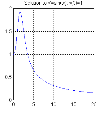
x'(t)=sin(tx(t)) with x(0)=1 for 0 < t < 20.
Solution: Create (click here
to learn how) the following M.file called
firstode.m:
function
xpr=firstode(t,x);
%This
M-file is used with ode45 to solve the differential equation
% x'(t)=sin(tx(t))
%
xpr=sin(t*x);
Save the result in the workspace. At the command line type:
EDU» [t,x]=ode45('firstode',[0,20],1);
EDU» plot(t,x)
EDU» grid on
EDU» title('Solution to x''=sin(tx), x(0)=1')
This will produce the following plot:


Example 2
Consider solving the second order ODE:
y''+y'+y=asin(t)
with y(0)=3 and y'(0)=2 (#)
Solution: First write the equation as a system of first order
equations as in the last assignment (7. ODE Systems.)
To do this, let x(1)=y and x(2)=y'
so that
x(1)' =
x(2) and
x(2)' = y'' = -y'-y+sin(t)
=
-x(2)-x(1)+sin(t)
(##)
In the M-file below, xpr will denote the column
vector
|x(1)|
|x(2)|.
We now encode the information about Equation (#) as
represented in Equation (##) in the following M-file
(click here
to learn how to make M-files) called secondode.m:

function xpr=secondode(t,x);
a=0;
xpr=[x(2);-x(2)-x(1)+a*sin(t)];
%
% Some comments which you do not need to copy into your M-file.
% a = the Amplitude of the forcing term which is taken to be zero.
% The third line defines the function. The output is a column vector.
% [a;b] is one of MATLAB's way of writing the column
vector
% |a|
% |b|.

After saving secondode.m in the work space we may type, at the command
prompt, the following lines:
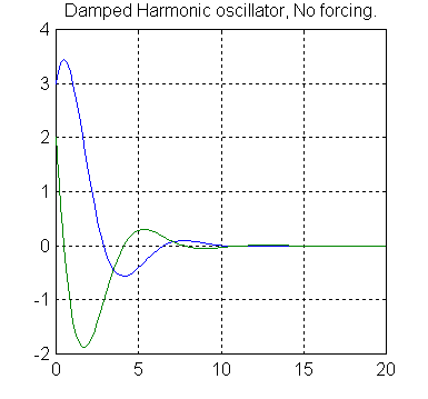
EDU» [t,x]=ode45('secondode',[0,20],[3,2]);
EDU» plot(t,x)
EDU» grid on
EDU» title('Damped Harmonic oscillator, No forcing.')
This will produce the following plot:

The blue line represents y(t) and green line represents y'(t).
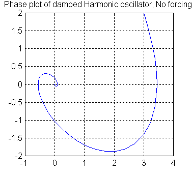
Typing
EDU» plot(x(:,1),x(:,2));
EDU» title('Phase plot of damped Harmonic oscillator, No forcing.')
EDU» grid on
produces the "phase space" plot of the solution: 
[Objectives | Exercises | Example
1 | Example 2
]
|