Perhaps the most natural notion of clustering in a graph is the clique number, namely, given a graph G what is the largest subgraph isomorphic to a complete graph? While much can be said deterministically (and even probabilistically), computing this statistic is generally very hard. However, the problem of determining large clusters remains of great interest.
One avenue to skirt the difficulty of computing clique number is to relax our problem to a similar, but more computationally tractable approach. Thus, we shall define a statistic known as the sigma-function of a graph, which we denote by σ(G). For our purposes, it suffices to note that the sigma-function gives a real value bounded between the clique and chromatic number. Further, the sigma-function arises from optimization over all positive edge-weightings of G.
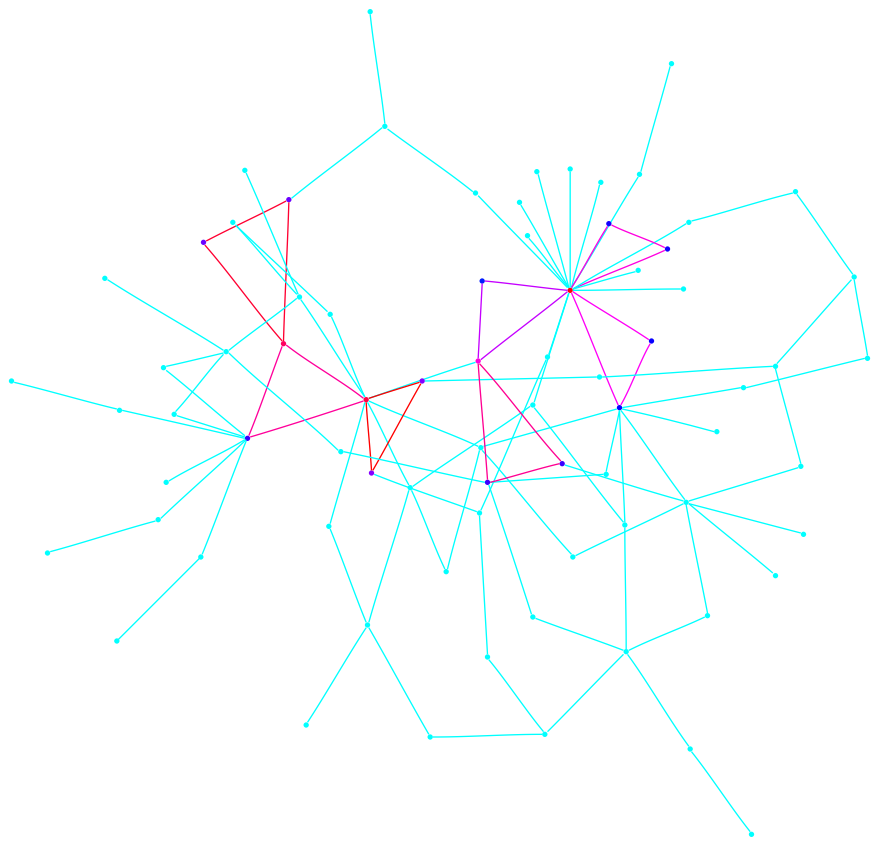
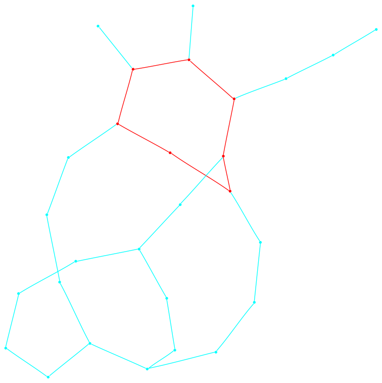
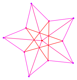
In what follows we present the sigma-function of each graph and a drawing. We indicate edge weights using the color scheme below; note that edge weights are normalized so that the largest weight always has value one. The reader who is interested in the definitions and analysis of the sigma-function are encouraged to see a paper co-authored with Fan Chung, found here. The Matlab™ code used to produce these graphs is found at the bottom of the page.
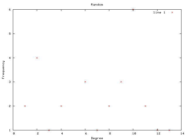
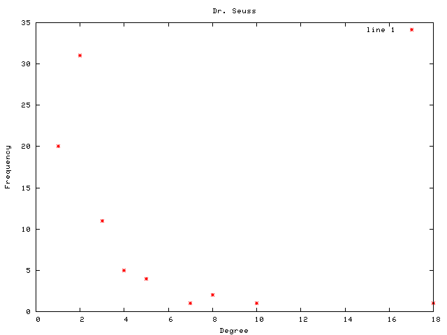
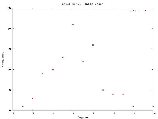
Each graph consists of a drawing (with weighting), a degree plot, basic statistics, and both a Matlab™ and Graphviz DOT file representation.
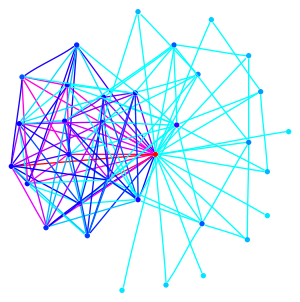
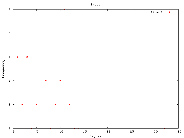
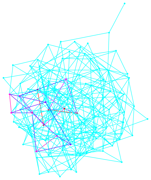
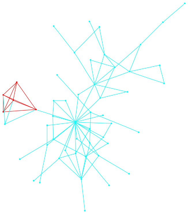
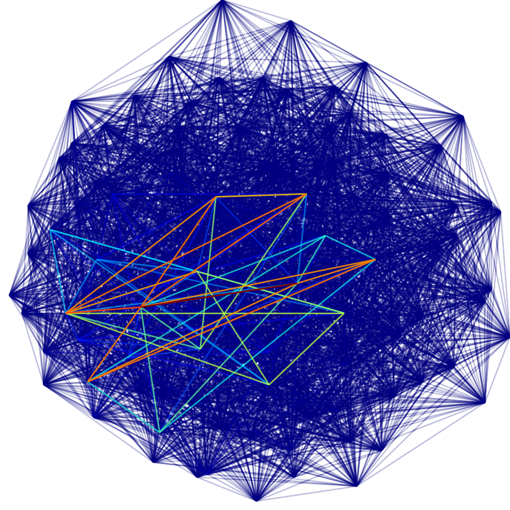 This graph is a large Payley which I ran a new iteration
of the sigma software on. It also demonstrates our new and improved
drawing code.
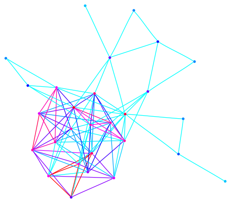
This graph is a large Payley which I ran a new iteration
of the sigma software on. It also demonstrates our new and improved
drawing code.
Here are the files used to compute the sigma-function and edge weights. A brief description of the formulæ involved can be found in the paper linked at the top of the page. Basically, this program solves an SDP (using the library SeDuMi) and converts the solution into a weight matrix.
To use the attached files, one would need to first install SeDuMi (found here) and have it accessible to Matlab™. Then, having all the below m-files in one place and available to Matlab, one need do the following to run an instance.
>> load example_graph;The result will be the weight matrix W, the corresponding Laplacian L, and the sigma value sigma. This algorithm works with sparse matrices; indeed, they are highly recommended. The last method, sigma_write_dot, is a utility routine for writing the graph with edge weights in GraphViz format (indeed, this is how the above images were produced). If you actually want to run this code, feel free to contact me, and I will give you further pointers. As you might expect, these files come with no warranty of any kind and no implied support. Use at your own risk.
>> [W, L, sigma] = sigma_calc_weights(example_graph, 0);
>> sigma_write_dot(example_graph, W, 'example.dot', 0, 0);