Systems of ODEs

At the end of Assignment 2, we created phase portraits using the commands phaseplane and drawphase in order to explore 2×2 systems of ODEs. In this lab, we will further investigate systems of equations and focus on linear ones, the advantages of specialization being that the techniques of eigenvalues and eigenvectors you will study here are extremely effective even for systems of large size. A homogeneous 2×2 system of linear ODEs has the form

(1)	`x′ = ax + by` `y′ = cx + dy`

where a, b, c, and d are constants.

To solve a system of linear differential equations, it is often helpful to rephrase the problem in matrix notation. The above system can be expressed as

v′ = Av

where v is the column vector and A is the matrix . Such systems can be solved using the eigenvalues and eigenvectors of the matrix A, as we shall see below. To begin wtih, let's look briefly at how matrices are entered and manipulated in MATLAB.

Matrices in MATLAB

To enter a matrix into MATLAB, we use square brackets to begin and end the contents of the matrix, and we use semicolons to separate the rows. The components of a single row are separated by commas. For example, the command

>> A = [1, 2; 3, 4]

will result in the assignment of a matrix to the variable A:

We can enter a column vector by thinking of it as an m×1 matrix, so the command

>> b = [1; -1]

will result in a 2×1 column vector:

There are many properties of matrices that MATLAB will calculate through simple commands. Most of this material is covered in Math 20F, but a few basic properties can be helpful to us in solving systems of differential equations.

Eigenvalues and Eigenvectors

An eigenvalue λ for the matrix A is related to its eigenvector b by the equation

Ab = λb.

MATLAB can be used to find the eigenvalues and eigenvectors of a matrix using the eig command. When applying the command by itself, as in eig(A), MATLAB will return a column vector with the eigenvalues of A as its components. For example, with our matrix A above, we get the following output:

>> eig(A)

ans =

    -0.3723     
     5.3723

If we also want MATLAB to calculate the eigenvectors of A, we need to specify two output variables. The command and its output are below:

>> [eigvec, eigval] = eig(A)

eigvec =

    -0.8246   -0.4160
     0.5658   -0.9094
     
eigval =

    -0.3723    0
     0         5.3723

As you can see, by using this command, we get two matrices as output. The first matrix, called eigvec, has the eigenvectors of A as its columns. The second matrix, eigval, has the eigenvalues of A on its main diagonal and zeros everywhere else. The eigenvector in the first column of eigvec corresponds to the eigenvalue in the first column of eigval, and so on.

Let B be the matrix .

Define the matrix B in MATLAB with the values above. Copy and paste the input and output from your command into your Word document.
Use the MATLAB commands to find the eigenvalues and eigenvectors for the matrix B. Copy and paste the input and output from your command into your Word document.

Now that we've seen how to use matrices in MATLAB, we should be ready to solve systems of equations such as (1) above.

Homogeneous Systems of Linear ODEs

As you have probably already seen in class, when the matrix A = has two distinct eigenvalues, the general solution to the system (1) is

(2)	`v(t) = c₁·e^λ₁·tb₁ + c₂·e^λ₂·tb₂,`

where λ₁ and λ₂ are the eigenvalues of A; the vectors b₁ and b₂ are the corresponding eigenvectors; and c₁ and c₂ are constants determined by the initial conditions. It is important to recognize that eigenvalues can be real or complex. In the remainder of this lab, we will examine how the eigenvalues of a linear system determine the behavior of the solution curves.

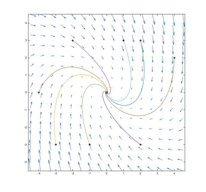
Real Eigenvalues

Let us begin by examining the familiar case when the eigenvalues are real.

Consider the system of differential equations

(3)	`^dx⁄_dt = -2.1x + 1.2y` `^dy⁄_dt = 0.8x - 3.4y`

When the system is put into the form v′ = Av, the matrix is given by A = . Enter this matrix into MATLAB with the command

>> A = [-2.1, 1.2; 0.8, -3.4]

We can get the eigenvalues and eigenvectors of A by typing

>> [eigvec, eigval] = eig(A)

eigvec =

     0.9159   -0.5492
     0.4013    0.8347
     
eigval =

    -1.5742    0
     0        -3.9258

Using the eigenvalues and eigenvectors listed above, we find the general solution:

We can tell quite a bit about the solution just by looking at it qualitatively. Since both eigenvalues are negative, and because they constitute the rate constants of the exponentials, the solution will tend to 0 as t gets larger regardless of which values we choose for c₁ and c₂.

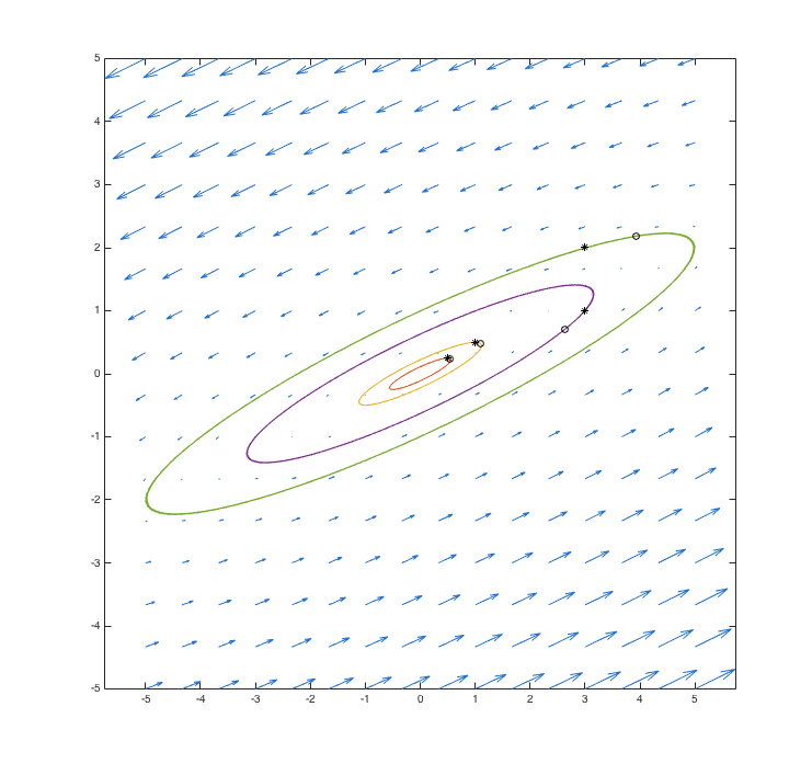
We can also get a visual representation of the solutions by using phaseplane and drawphase. (Revisit Assignment 2 for more information about these commands.)

>> g = @(t,Y) [-2.1*Y(1) + 1.2*Y(2); 0.8*Y(1) - 3.4*Y(2)];
P = [-3,3; -3,0; -3,2; -2,-3; -1,3; 0,-3; 1,4; 2,-3; 4,-2; 4,0; 4,2];
phaseplane(g, [-4.5,4.5], [-4.5,4.5], 16)
hold on
for i=1:size(P,1)
    drawphase(g, 50, P(i,1), P(i,2))
end
hold off

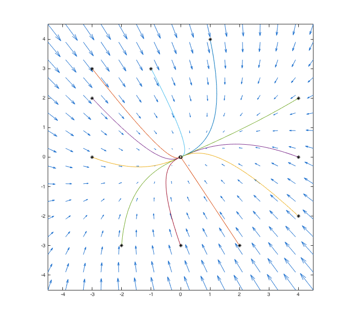
Just as we predicted by looking at the eigenvalues, all the solutions shown here tend to 0. (The endpoints of each curve at our final time, in this case at t = 50, are marked with circles. These are not actually at the origin, but they are very, very close, which is why they all overlap.)

You should take a moment to look at these commands and make sure you understand how they work. Some things you might want to determine:

What does the function g represent? [Hint: Y(1) refers to our first dependent variable, which in this system is x.]
What is P, and how was it used? Try copying and pasting this code into MATLAB and then changing a few of the entries of P or adding new rows. Then run the commands and see what happens.
What did our for loop do?

Now that we've seen an example, you're going to try all this on your own.

Consider the system of differential equations

(4)	`^dx⁄_dt = 3x + 4y` `^dy⁄_dt = -x - 2y`

When the system (4) above is put into the form v′ = Av, what is the matrix A? Enter the matrix A into MATLAB, and record the input and output for this in your Word document.
Use MATLAB to find the characteristic roots (eigenvalues) and characteristic vectors (eigenvectors) of your matrix A. Copy and paste all input and output from your command into your Word document.
Use the formula (2) above and the results from part (b) to write the general solution of our system (4). Write this solution in your document. What happens to the system as t gets large?
Use phaseplane and drawphase to create a phase diagram of the solutions. Make sure you draw at least six solution curves. (You may want to simply modify the code from the example.) Include this plot in your writeup. Does the plot support your answer to (c)?

Complex Eigenvalues

In our 2×2 systems thus far, the eigenvalues and eigenvectors have always been real. However, it is entirely possible for the eigenvalues of a 2×2 matrix to be complex and for the eigenvectors to have complex entries. As long as the eigenvalues are distinct, we will still have a general solution of the form given above in (2). In order to build up an understanding of this equation, we will take a brief detour for a review of complex exponentials and of complex numbers more generally.

If our system has complex eigenvalues, then formula (2) tells us we will have to deal with complex exponentials. Recall that if c = a + ib, then we can write e^ct = e^ate^ibt. Splitting up the exponential like this helps us to see how the real and imaginary parts of c affect the exponential.

If a < 0, then the function e^at will damp out as t grows larger. If, on the other hand, a > 0, then e^at will cause the exponential to explode when t gets big.

The purely complex part, the e^ibt, has absolute value one; as t changes, this part of the exponential will move along a circle when plotted in the complex plane. The larger b is, the faster the function circles.

Let's review the relationship between a complex number and its real part. Given the complex number c = a + ib, its complex conjugate is given by c̄ = a - ib. The real part of c equals ^{(c + c̄)}⁄₂.

We shall be interested only in real-valued functions v(t). In formula (2), v(t) is real if and only if the second term is the complex conjugate of the first. Thus, if we have a 2×2 system with complex eigenvalues c = a + ib & c̄ = a - ib and corresponding eigenvectors u & ū, then (2) is given by

v(t) = c₁·e^ctu + c₂·e^c̄tū = d₁·Re(e^ctu) + d₂·Im(e^ctu).

Note that Re here is a function that takes the real part of a complex number, and Im takes the imaginary part. If we look only at the first term of the above, we see that this can be written as

v(t) = e^at·Re(e^ibtu).

Let's get some practice seeing what these individual solutions look like.

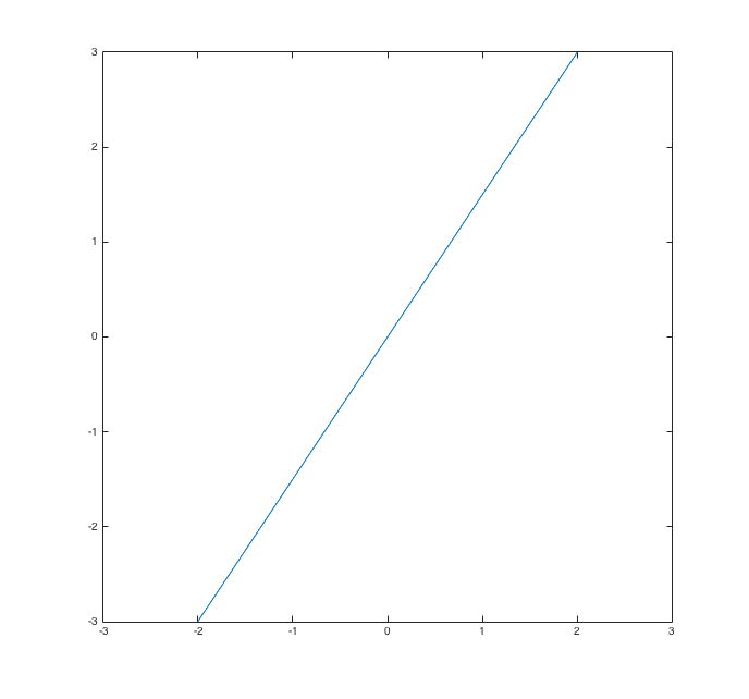
Consider the exponential given by . The parametric graph of this is printed below.

The vector itself can be complex, as in the function , which has graph

In typical practical problems, data and measurements consist of real numbers rather than complex numbers. However, when we solve for the eigenvalues and eigenvectors of A, we may get complex values, which seems counterintuitive. The following theorem makes sense of this.

Theorem 4.1. If the entries of A are real numbers and the initial condition is a vector with real entries, then the solution v(t) is a vector with real entries.

Let us see what algebraic structure this theorem actually provides. Suppose that the matrix A has an eigenvector b with corresponding eigenvalue λ, so that Ab = λb. One consequence of the theorem is that the complex conjugate of b is also an eigenvector, and its corresponding eigenvalue is the complex conjugate of λ. This behavior ensures that even when the eigenvalues and eigenvectors have complex numbers in them, the solutions will still be real-valued.

The conclusions of this theorem can be very deceptive! Many students try to conclude that because the solutions will be real, we can ignore complex numbers. This is not true! As we will see later, complex eigenvalues lead to solutions that "spiral." Indeed, complex numbers arise any time we have a system of differential equations describing oscillatory motion.

Now that we've built up our understanding of complex exponentials, let's do an example applying them to a 2×2 system.

Consider the system of differential equations

(4)	`^dx⁄_dt = -0.5x + 0.9y` `^dy⁄_dt = -1.2x - 1.7y`

Putting the system in the form v′ = Av, we get the matrix A = . As before, once we define the new matrix A in MATLAB, we can use the program to calculate the eigenvalues and eigenvectors.

>> [eigvec, eigval] = eig(A)

eigvec =

    -0.3780 - 0.5345i   -0.3780 + 0.5345i
     0.7559             -0.7759
     
eigval =

    -1.1000 + 0.8485i    0
     0                  -1.1000 - 0.8485i

We have learned that the general solution in (2) is still valid for complex eigenvalues and eigenvectors. Hence, the general solution here is

Now we'll plot solutions using phaseplane and drawphase:

In the last example, the solutions once again tended to zero as t increased. That is not always the case.

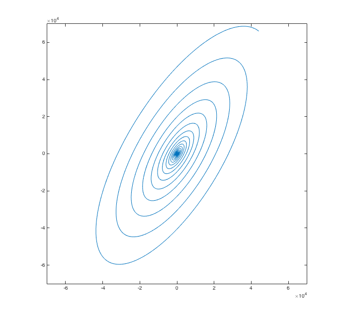
Consider the system of differential equations

(6)	`^dx⁄_dt = 2.7x - y` `^dy⁄_dt = 4.1x + 3.7y`

Put the system above in the form v′ = Av and enter the matrix A into MATLAB. Use MATLAB to find the eigenvalues and eigenvectors of A. Copy and paste all input and output from your command into your Word document.
Write the general solution of the system (6) in your Word document.
Use phaseplane and drawphase to create a phase diagram of the solution. Make sure to draw at least six different curves using drawphase. Include the resulting plot in your writeup. Which feature of the eigenvalues or eigenvectors causes the solutions to tend to infinity as t grows large?

Higher-Dimensional Systems

So far, our discussion has focused only on 2×2 systems. While we are unable to plot larger systems, our analysis of the eigenvalues still allows us to analyze their behavior. For instance, a 4×4 matrix A with real entries typically has four eigenvalues λ₁, λ₂, λ₃, and λ₄, with eigenvectors b₁, b₂, b₃, and b₄, respectively. These correspond to solutions of the form

v(t) = c₁·e^λ₁tb₁ + c₂·e^λ₂tb₂ + c₃·e^λ₃tb₃ + c₄·e^λ₄tb₄

The solution is real-valued, and its form depends on how many of the eigenvalues are real. For example, if λ₁ and λ₂ are real but λ₃ and λ₄ are complex, then λ₃ and λ₄ are complex conjugates to each other, and all real solutions have the form

v(t) = c₁·e^λ₁tb₁ + c₂·e^λ₂tb₂ + c₃·Re(e^λ₃tb₃) + c₄·Im(e^λ₄tb₄)

Another possibility is that none of the eigenvalues are real, so that we have two pairs of complex conjugates. Suppose λ₁ is conjugate to λ₂ and λ₃ is conjugate to λ₄. Then our solution will have the form

v(t) = c₁·Re(e^λ₁tb₁) + c₄·Im(e^λ₂tb₂) + c₂·Re(e^λ₃tb₃) + c₄·Im(e^λ₄tb₄)

What about when λ₁ is real and λ₂, λ₃, & λ₄ are not real? Is this possible?

Stability

One of the most important properties one worries about when dealing with situations governed by differential equations is whether or not the system is stable. To use a bit of hyperbole, if you were to buy a piece of electronics that was not stable, it might blow up when you plug it in, or else it might produce large and unwanted oscillations. Stability is not limited to electronics, however. Economic models can become unstable, as was seen in the financial meltdown of September 2008. Even designers of algorithms worry about the stability of their algorithms; from a mathematical point of view, convergence of an algorithm amounts to a type of stability. And you can think of stability in physical terms as well, as we will when we consider an airplane's sensitivity to turbulence.

Definition 4.1. In the realm of differential equations, a linear system v′ = Av is called stable when every solution v(t) stays bounded as t tends to infinity. A linear system is called asymptotically stable when every solution v(t) tends to zero as t tends to infinity. (Asymptotic stability is stronger than stability; that is, if a system is asymptotically stable, then it is stable.)

In this section, we will examine stability for linear systems, and we will see how we can use the eigenvalues of a system to determine whether it is stable, asymptotically stable, or unstable. We will start with 2×2 systems, and then we will indicate how our analysis scales to systems of any size.

In Example 4.1, we saw that the system given by (3) had eigenvalues -1.5742 and -3.9258. The analysis given there and the phase portrait of the direction field both showed that all the solutions tended to 0 as t got large. Thus (3) is an example of an asymptotically stable system. In fact, a system is asymptotically stable if and only if the eigenvalues of that system are both negative.

Contrast this with Exercise 4.2, in which you saw how the solutions to the system (4) got larger as t tended to infinity. This is an example of an unstable system. Take a look at the eigenvalues for this system: 0.6533 and -7.6533. Any system with even one positive eigenvalue will be unstable.

For an additional example, consider the system given by

(7)	`^dx⁄_dt = 2x - 5y` `^dy⁄_dt = x - 2y`

The phase diagram for this system looks like

Notice that the solution curves on this plot do not approach zero, but they do remain bounded. That makes this an example of a stable system that is not asymptotically stable. MATLAB tells us that the eigenvalues of this system are i and -i. The key here is that there is no real component to the eigenvalues. Can you see, in terms of the formula (2), how this determines the behavior of the solutions?

The takeaway here is that the eigenvalues determine the stability (or otherwise) of a system. There are two important things to note. First, we have not considered all possible cases for the eigenvalues. Second, while phase portraits are helpful for 2×2 systems, we cannot plot larger systems. That means we must look at our solution from (2) and do our analysis directly. We have the following theorem to help us deternmine the stability.

Theorem 4.2. For a linear system v′ = Av of dimension n, suppose the eigenvalues of A are λ₁, ···, λ_n.

The sysmtem is asymptotically stable if and only if Reλ_i < 0 for all i;
Suppose A is diagonalizable. Then the system is stable if Reλ_i ≤ 0 for all i.

The theorem above is not in the most general form due to the scope of this course. However, it is useful in most of our cases. Note that when the matrix produced by eigvec is nonsingular, A must be diagonalizable.

Consider the 3×3 system

(8)	`^dx⁄_dt = 1.25x - 0.97y + 4.6z` `^dy⁄_dt = -2.6x - 5.2y - 0.31z` `^dz⁄_dt = 1.18x - 10.3y + 1.12z`

Define the matrix A in MATLAB with the values above, using A = [1.25, -0.97, 4.6; -2.6, -5.2, -0.31; 1.18, -10.3, 1.12], and calculate the eigenvalues of A. Copy and paste the input and output from MATLAB.
Using your answer from part (a), is the system in (8) stable? Justify your answer.

Application: Airplane Controls

One fundamental property of all linear dynamical systems (meaning most objects that move) is that they have resonances. These are associated with eigenvalues and eigenvectors of the coefficient matrix of the system. While we could illustrate this with fluids in pipes, electrical circuits, signals in the air, the effects of earthquakes on buildings, and more, we have chosen to illustrate this property with an airplane. This particular example is both familiar and easy to visualize.

Before we begin, we'll introduce some terminology. When we examine the flight dynamics of an aircraft, we're usually concerned with three types of rotation: pitch, roll, and yaw. Pitch is the angle of rotation associated with the rise and fall of the nose of the aircraft, either pointing up or down. Roll is the angle by which the wings deviate from being level, so that one wing rises up and the other drops down. Yaw refers to rotation around a vertical axis, moving the nose of the airplane left or right; a change in yaw results in a change of heading for the plane. Take a look at the animated images below, and try to identify the three different kinds of rotation.

These images are provided by NASA and are in the public domain.

We will consider a model used in the design of commercial aircraft. This is a differential equation that describes the effect of rate of change of rudder angle on the rate of change in yaw. The yaw rate model is the 4×4 system

(9)	`x′(t) = Ax(t) + Bu(t)`

with a single function u as the driving term. Here, u is the rate of change of rudder angle, and the four components of x are:

x₁ = lateral (side-to-side) velocity;
x₂ = yaw rate;
x₃ = roll rate;
x₄ = pitch rate.

A is the 4×4 matrix , and B is the 4×1 matrix .

In our exercise we will ignore the effects of the driving term and instead consider the homogeneous system x′ = Ax. In effect, this means our aircraft has no control system. We'll see very soon that such an airplane couldn't fly for long.

Define the matrices A and B in MATLAB:

>> A = [-0.0558 -0.9968 0.0802 0.0415;
0.598 -0.115 -0.0318 0;
-3.05 0.388 -0.465 0;
0 0.0805 1 0]

>> B = [0.01; -0.175; 0.153; 0]

What are the eigenvalues and eigenvectors of the matrix A? Include your input commands and your output in your Word document.
According to the mathematical definitions, is the system x′ = Ax stable, asymptotically stable, or unstable? Why?
One of the eigenvalues you obtained is very close to zero. Look at the corresponding eigenvector. Which component is biggest? Based on that, which type of rotation is this eigenvector most closely associated with: yaw, roll, or pitch?

You may find the practical implications of the eigenvalue locations interesting:

There are two real eigenvalues, and one of them is sufficiently negative that its effect damps out quickly. Indeed, this eigenvalue has little effect on the performance of the airplane.
The other real eigenvalue is close to zero and real. This corresponds to the responsiveness of the airplane to the pilots' commands, which is very desirable. Since there is no imaginary part, no oscillation occurs.
There is a conjugate pair of complex eigenvalues (call them c and c̄) close to the imaginary axis. Even though their real part is negative, it is so small that their effect damps out slowly. These eigenvalues correspond to a basic tendency for the airplane to oscillate left and right and roll at speed equal to Im(c) radians per second. This is called the Dutch Roll Mode, and it can be very bad. A wind gust might "excite" the Dutch Roll Mode, and then another gust might well increase it.

These three effects collectively are called the resonant modes or eigenmodes of the airplane.

This illustration of Dutch roll was made by Wikipedia user Picascho and is in the public domain.

Controlling the Dutch Roll

Fortunately, as we mentioned before, this is a model of an airplane with no control system. Based on this mathematical model, engineers design and implement a control algorithm called a yaw damper that automatically moves the rudder back and forth and compensates for this phenomenon. Large commercial airplanes require a yaw damper.

Exactly what is involved in designing this control system? At any time t, sensors tell us the state x(t) of the plane, and (roughly speaking) we can at that time ensure that that the rate of change of rudder angle u(t) is whatever we want. Let us make it a simple function of the form

u(t) = Fx(t) + u_p(t)

where F = [F₁ F₂ F₃ F₄] is a 1×4 matrix. Here, u_p(t) represents the pilot's instructions to the rudder, and the product Fx(t) is what the plane's computer tells the rudder to do in order to damp the plane's bad resonant oscillations.

In this scenario, our design amounts to choosing the entries of F: F₁, F₂, F₃, and F₄. Putting this together with the airframe model given by (9), we get

x′(t) = Ax(t) + B(Fx(t) + u_p(t)) = (A + BF)x(t) + Bu_p(t).

The stability of this system is completely determined by the eigenvalues of (A + BF).

Recall that we specified A as and B as .

If F = [0 7 0 -1], what is the matrix BF?
If F = [0 5 0 -0.1], what is the matrix BF?
If F = [0 5 0 -0.1], what is the matrix A + BF? Are its eigenvalues the same as or different from those of A?
Find F = [F₁ F₂ F₃ F₄] such that the damping of yaw oscillation is increased and the plane still responds decently to pilot commands. More specifically: we want the complex eigenvalues to have real part less than -0.2, and we want there to be a real eigenvalue within 0.02 of zero. [Hint: There is a solution with F₁ = 0 = F₃ and F₄ = -0.09, so you only need to fiddle with F₂ to find an appropriate value.]

Ultimately, the goal of this exercise is not to design a real control system, but rather to demonstrate that eigenvalues and eigenvectors are associated with basic behaviors (the resonant modes) of the airplane. This is true not just for mechanical objects but also for anything else that changes with time. If we understand one example, such as this airplane situation, we can apply our understanding to many other areas.

Conclusion

Systems of differential equations constitute the mathematical models central to many technological and scientific applications. In practice, models requiring many differential equations are much more common than models using only one. It's not unusual to use dozens of variables. In this lab, we saw how matrices and a little bit of linear algebra can give us powerful tools for working with linear systems, even very large ones.

Later in class you will study Laplace transforms. For linear systems, they combine very well with the linear algebra techniques we have seen here, producing some of the main design techniques used in engineering.

Last Modified: 8 January 2017